
Introduction
- An end-to-end transformer model, conceptually similar to Stable Diffusion or GPT but applied to a different task.
- It takes a sequence of images as input.
- It outputs camera poses, depth maps, point maps, and tracking information.
- It can process hundreds of images within one second.
- It infers the complete set of 3D attributes without requiring post-optimization.
Background
-
Traditional 3D reconstruction utilize visual-geometry methods (BA)
BA (Bundle Adjustment) is a mathematical optimization technique to refine the 3D structure and camera positions by minimizing reprojection errors across multiple views. 最小化重投影误差LM算法使得观测的图像点坐标与预测的图像点坐标之间的误差最小
-
Machine learning method: address tasks like feature matching and monocular depth prediction
-
VGGsfm: integrate the deep learning model into the SfM(structure from motion) to achieve end-to-end
-
VGGT: predicts a full set of 3D attributes, including camera parameters, depth maps, point maps, and 3D point tracks.
Tracking Any Point: track the POI in the video sequence
Model Architecture
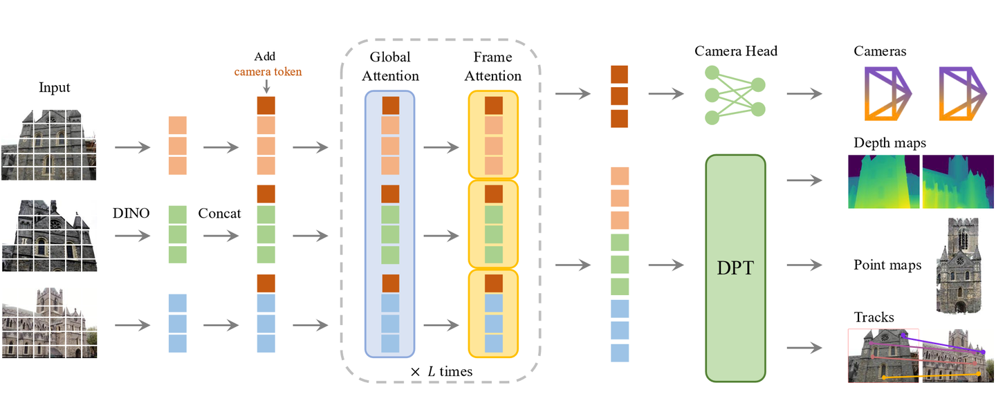
Aggregator
The model first processes input images using an aggregator.
- DINO: Used for image patchification to get local tokens ().
- Augmentation tokens:
- A camera token () is added.
- A register token () is added.
- Concat: The tokens are concatenated, and positional embeddings are added.
Alternating Attention
The token sequence is processed through L layers of alternating attention blocks.
- Global Attention: Attention is computed across tokens from all frames. Tensor shape: [B, N*P, C].
- Frame Attention: Attention is computed among tokens within each individual frame. Tensor shape: [B*N, P, C].
The initial camera token () and register token (t_1R) are learnable, allowing the model to set the first frame as the coordinate system. The register token (t_R) is discarded during the prediction phase.
Prediction Heads
After the attention blocks, the tokens are passed to different prediction heads to generate the final outputs.
- Camera Head:
- Uses the camera token (t_ig).
- Predicts the camera parameters (g) using self-attention and a linear layer.
- DPT Head:
- Uses the image tokens (t_iI).
- Employs a DPT (Dense Prediction Transformer) to get feature maps F_i (with shape CxHxW).
- A 3x3 convolution predicts the depth map (D_i), point map (P_i), tracking features (T_i), and a confidence map.
- Track Head:
- For a given query point (y_j) in a query image (I_q).
- It performs a bilinear sample on the feature map (T_q) to get the feature (f_y).
- This feature is correlated with other feature maps (T_i) to get correlation maps.
- These maps are fed into a self-attention layer to predict the corresponding 2D points (y_i).
Training
The model is trained with a composite loss function. The camera loss uses the Huber Loss function.
-
Total Loss:
-
Camera Loss:
-
Depth Loss:
-
Point Map Loss:
-
Track Loss:
Limitations
- Does not support fisheye or panoramic images.
- Reconstruction quality is low when input images have extreme rotations.
- Inference memory usage increases rapidly as the number of input images grows.